

[Project Notes] RL in a World Model, in Rust: What Our Pushing Experiments Taught Us
Published:
One result changed how I looked at this project: a policy trained from scratch inside our world model reached 82% predicted success, then 0% success when evaluated in the physics simulator. The imagined task looked solved. The pushing task wasn’t.
I built RL-in-WM-in-Rust to test a small version of an appealing loop: train a policy, collect its experience, learn a world model, and use that model to train a better policy. A two-joint arm pushing a block seemed simple enough to make the whole experiment inspectable on a Mac. It also made a useful failure visible: a model that predicts recorded trajectories reasonably well can still be a poor environment for optimizing a new policy.
These notes describe the implementation and the experiments recorded on September 10, 2026, at repository commit 778309b. Throughout this post, “real” means the analytic physics simulator, used as our reference environment. We have not tested a physical robot.
A small task with separate stages
The arm has a fixed base and two revolute joints. The block and goal positions vary between episodes, but the reset distribution is structured: they lie on the same circle around the base, with radius 0.95–1.20 and a goal-angle offset of 0.50–0.62 radians. This is not a benchmark over arbitrary reachable block–goal pairs. The simulator runs four 60 Hz substeps per policy decision, giving a 15 Hz decision rate and a maximum episode length of 75 decisions, or five seconds. Success requires keeping the block within 0.07 distance units of the goal for at least 0.25 seconds. Contact is approximated with a disk-shaped block; this is a lightweight test environment, not a high-fidelity rigid-body engine.
I wanted to inspect the boundary between each stage, so the Rust version writes explicit artifacts:
flowchart TD
    A["Physics simulator + PPO"] --> B["Policy checkpoint"]
    B --> C["Collect complete trajectories"]
    C --> D["Dataset: state, action, next state"]
    D --> E["Train dynamics ensemble"]
    E --> F["Compare predicted and recorded trajectories"]
    E --> G["PPO inside the world model"]
    B -. "optional fine-tuning initialization" .-> G
    G --> H["Evaluate in the physics simulator"]
    H -. "proposed next iteration" .-> C
The final feedback edge is a research plan, not an automatic improvement loop already implemented in the repository. Collection, dynamics training, model PPO, and evaluation are separate CLI commands. That makes it possible to replace a model while keeping the policy or evaluation dataset fixed.
The workspace contains five crates: env for physics, rl for neural networks and PPO/SAC, world for learned dynamics, cli for the experiment stages, and bench for throughput measurements. PPO samples environments in parallel with Rayon. The current SAC CLI advances its environments serially. Everything trains on the CPU; there is no Metal, MPS, or CUDA backend. For this small task, keeping the full learning loop easy to inspect mattered more to me than introducing a larger framework.
The policy chooses an action; the world model predicts a state
Our policy and world model have different jobs:
observation = encode(state)
action      = policy(observation)
next_state  = world_model(state, action)
reward      = task_reward(state, next_state, action)
The default policy receives 16 observation values: joint angles and velocities, block and goal positions, relative positions, block velocity and angular velocity, and episode time. Its PPO actor and critic are separate MLPs with two 32-unit tanh hidden layers. The actor produces two Gaussian means and two log standard deviations; actions are bounded with tanh.
The dynamics ensemble receives the 18-dimensional full state plus the two-dimensional action. Full state also includes controller targets, controller velocities, block orientation, and the success timer. Each member learns deltas for the first 14 state fields. Goal coordinates stay fixed, time advances analytically, and the model-environment adapter updates the success timer. Reward is computed from the predicted transition rather than learned by a separate reward network. The adapter implementation makes this boundary explicit.
To predict farther ahead, we feed the predicted state back into the policy, obtain another action, and call the world model again. The world model does not decide the next action. In a trajectory-comparison experiment, we instead replay a fixed sequence of recorded actions through the model, so action selection does not confound the dynamics comparison.
That distinction explains why a good-looking replay is not enough. During optimization, the policy can choose actions unlike those used to collect the dataset.
The first benchmark went backward
Our standard training scale is 13 parallel environments and 1,000 real PPO updates, with 256 decisions per environment per update: about 3.33 million transitions. For dynamics, the working configuration is 4,000 trajectories, 10 epochs, and three ensemble members. The recorded dataset contains 146,761 transitions and is split by complete episode into training, validation, and test partitions.
The first comparison used 100 physics-simulator episodes with seeds 80000–80099 and deterministic policy actions:
| Policy | Initialization | Simulator success |
|---|---|---|
| Real PPO | Trained in the physics simulator | 85% |
| World-model fine-tuned PPO | Loaded the real PPO checkpoint | 54% |
| World-model cold-start PPO | Random network initialization | 0% |
These are measurements from one experimental setup, not multi-seed algorithm averages. The recorded benchmark summary preserves the evaluation conditions and return metrics.
The mismatch also appears in a separate paired diagnostic. Starting from the same 100 initial seeds, 29000–29099, real PPO scored 65% in the model and 82% in physics; the fine-tuned policy scored 69% and 57%. The model could underestimate one policy and overestimate another. These starts came from the data-collection seed range, so this diagnostic should not be presented as a new held-out generalization benchmark.
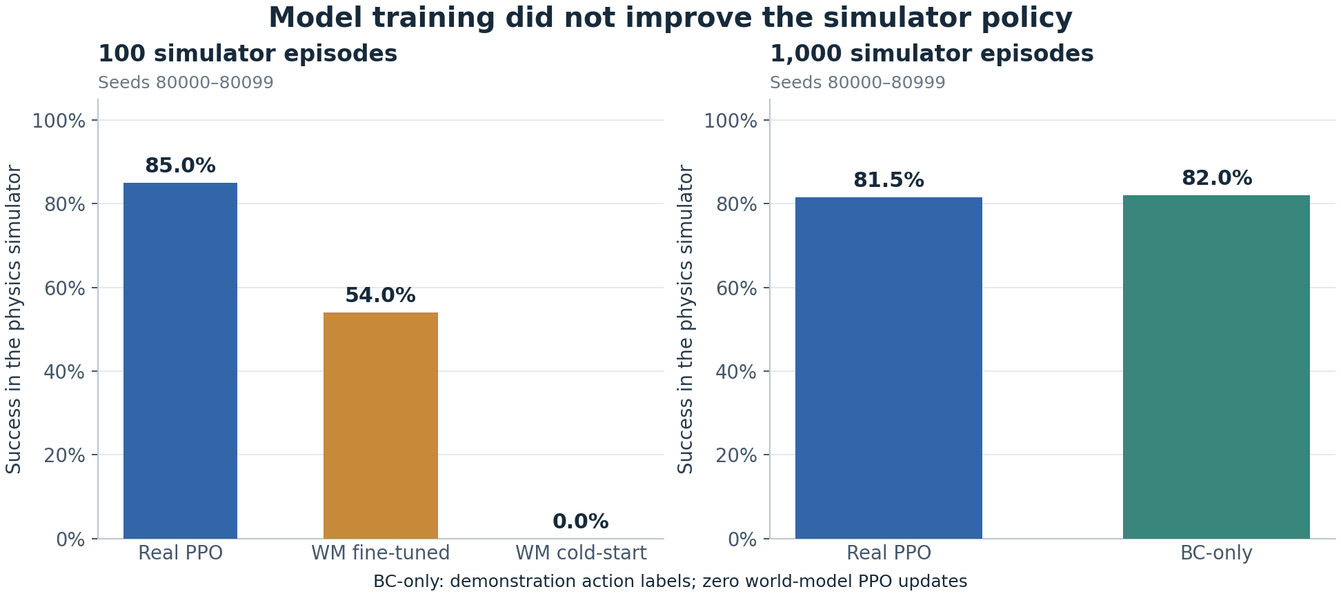
The left panel uses 100 simulator episodes, seeds 80000–80099. The right panel uses 1,000 episodes, seeds 80000–80999. BC-only uses action labels and zero model PPO updates. The evaluation prefixes overlap; the panels are not independent replications.
Our interpretation is that PPO is exploiting errors in the learned dynamics. The implementation offers a plausible mechanism: reward increases when the predicted block moves toward the goal, but the learned transition has no hard constraint requiring a physically valid arm–block contact. An impossible but rewarding transition can therefore look attractive to the optimizer. This is a hypothesis supported by the model/physics gap and the code structure; we have not isolated every contribution with a controlled ablation.
Thirty steps cover two seconds, not the entire task
I initially wondered whether a model needed to predict all 75 steps before RL could learn to finish. A short rollout can still contribute to a longer-horizon policy. At a truncation, the value function estimates what comes afterward. For example, a 30-step target has the form
\[\hat G_t=\sum_{k=0}^{29}\gamma^k r_{t+k}+\gamma^{30}V(\hat s_{t+30}).\]That final value is an estimate, not missing ground truth. It must itself be learned from useful states. We therefore tried resetting model rollouts to states sampled throughout recorded trajectories, including later phases, rather than always restarting at the beginning. In this implementation, the reset jumps to a recorded state; it does not query the simulator for a fresh observation every 30 steps or guarantee continuous physical progress.
This was inspired by the short model rollouts branched from real data in MBPO. Our experiment is a PPO variant borrowing that idea, not a reproduction of the complete MBPO algorithm.
With 500 model PPO updates, the 30-step episode-start variant reached 21% simulator success. Sampling replay starts raised it to 35%; a 45-step replay variant reached 27%. All three started from the real PPO checkpoint. They are fine-tuning experiments, and all remained below the original 54% model fine-tuning result in the 100-episode benchmark.
Changing rollout usage also does not change the weights of a frozen world model. After we separately collected new data from the short-rollout policies and retrained dynamics, their step-30 full-state MSE values were about 0.432 and 0.776, compared with 0.232 for the standard model on the same held-out cohort. The short-rollout intervention did not automatically improve dynamics accuracy.
More data and fewer epochs did not improve every metric
For a more careful dynamics comparison, we collected 1,000 evaluation trajectories with seeds 900000–900999 and selected the 299 trajectories that lasted at least 30 steps. Every model used that same cohort and the same recorded actions, predicting autoregressively without teacher forcing. This avoids silently changing the population as the plotted horizon grows, although it excludes episodes that finish early.
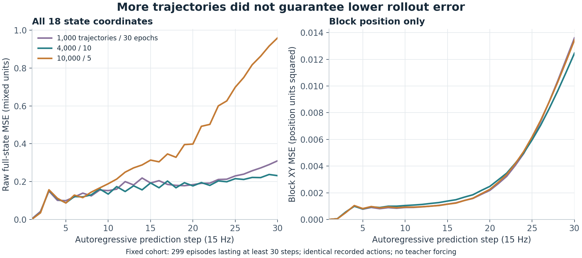
Left: raw MSE across the 18 state coordinates, which mix physical units. Right: block XY MSE, in squared position units. Both panels use the same 299-episode cohort. Curve data and evaluation protocol.
| Dynamics training configuration | Full-state MSE at step 30 | Block XY MSE at step 30 |
|---|---|---|
| 1,000 trajectories / 30 epochs | 0.3102 | 0.01361 |
| 4,000 trajectories / 10 epochs | 0.2315 | 0.01246 |
| 10,000 trajectories / 5 epochs | 0.9596 | 0.01345 |
This is why we kept 4000/10 as the working configuration. It is the best of these three configurations on this diagnostic, not a universal optimum. Data volume and epochs changed together, so the comparison does not isolate the causal effect of either one. The relatively small differences in block-position error also tell a different story from the full-state aggregate.
Lower MSE is useful only after fixing the state scaling, evaluation data, horizon, and rollout protocol. Even then, average prediction accuracy does not establish policy quality. A model can be accurate on frequently observed motion yet wrong around the contact transitions that decide whether a push succeeds. Optimizing a policy actively searches for high-reward states, including states where the model has little support.
The 82% policy was an imitation baseline
The strongest new policy came from behavior cloning (BC). We initialized a fresh network, used the recorded action labels for 20 epochs, and set model PPO updates to zero. With the existing stride sampler, a requested cap of 120,000 selected 73,381 transitions from the 146,761-transition dataset.
One initialization seed achieved 86% on 100 simulator episodes, 82.8% on 500, and 82.0% on 1,000. The original PPO checkpoint achieved 81.5% on the same 1,000 episodes. Both results were reproduced after extracting the code into the standalone repository; the checkpoints and confirmation metrics are included.
This result needs a precise label. BC did not load the PPO weights, but it did use the PPO policy’s demonstrations. With zero model PPO updates, it is not evidence that cold-start RL inside the world model reached 82%. Nor does the 0.5-percentage-point difference establish an improvement over real PPO. The seed sweep and repeated use of evaluation prefixes also limit what we can infer from the best observed run.
Continuing PPO inside the model damaged the BC initialization:
| Experiment | Simulator success, 100 episodes |
|---|---|
| BC20 + 50 model PPO updates | 29% |
| BC20 + 500 model PPO updates | 17% |
| BC20 + 100 updates, uncertainty penalty 1 | 11% |
| BC20 + 500 updates, uncertainty penalty 3 | 34% |
The penalty idea follows MOPO, which penalizes model rewards using dynamics uncertainty. Here we used ensemble disagreement as a practical proxy. It was not calibrated to transition error, and several ensemble members can agree on the same wrong prediction. These tests show that our chosen penalty settings were insufficient; they do not refute uncertainty-aware model-based RL.
The experiment log records 19 configurations and two larger-evaluation confirmations. In its main matrix, model success uses dataset starts from seed 29000 while simulator success uses seeds from 80000. Those columns are not episode-paired; a separate file records the paired diagnostic. Keeping that distinction in the log matters as much as keeping the scores.
What would count as a useful next iteration
I would now prioritize testing whether model errors are small where the candidate policy actually goes. New simulator data should cover failed pushes, unusual contacts, and states reached by the new policy. Then I would retrain the model, constrain how far policy updates can depart from supported behavior, and evaluate every candidate in physics with the same data and compute accounting as the baseline.
That loop could improve a policy, but the current experiment has not demonstrated a self-improving cycle. Short rollouts, value bootstrap, and uncertainty guards help define where to trust a model; none provides new physical evidence by itself. On a task whose analytic simulator is already cheap, I also want any model-based method to justify its total wall-clock cost. Faster synthetic sampling would not be enough if it produced a worse policy.
For a quick local reproduction, the repository includes the real PPO and BC checkpoints:
git clone https://github.com/DavidLXu/RL-in-WM-in-Rust.git
cd RL-in-WM-in-Rust
cargo run --release -p push-cli -- \
  --evaluate --policy-checkpoint checkpoints/ppo-1000.json \
  --episodes 1000 --eval-seed 80000 --trajectory runs/eval-ppo.json
open visualize.html
On macOS, the last command opens the replay page; load runs/eval-ppo.json there. Substitute checkpoints/bc20-seed1.json to inspect the imitation baseline. The README contains the separate training stages. The next result I want is a policy that improves in the simulator after model-based training, under a clearly stated data budget, rather than another increase in imagined success.